Continuous Compounding: Unlocking Exponential Growth
Continuous compounding represents the theoretical limit of compounding frequency. Imagine earning interest not just annually, monthly, or even daily, but constantly, every infinitesimal moment. While practically impossible to achieve in its purest form, it serves as a powerful tool for understanding and approximating investment growth. The core concept revolves around reinvesting interest earned instantaneously back into the principal. This constant reinvestment fuels an accelerated rate of return compared to discrete compounding periods (e.g., annual, quarterly). The formula for continuous compounding is elegantly expressed as: A = Pert Where: * **A** represents the final amount after time *t*. * **P** is the initial principal balance. * **e** is the mathematical constant approximately equal to 2.71828 (Euler’s number). * **r** is the annual interest rate (expressed as a decimal). * **t** is the time in years. Let’s break down why this yields such powerful growth. With discrete compounding, interest is calculated and added at specific intervals. During the intervening period, the new balance doesn’t earn interest on the newly added interest. Continuous compounding eliminates these gaps. The smaller the compounding period, the closer it gets to continuous compounding, and the greater the return. The significance of ‘e’ is also crucial. It emerges naturally in calculus when dealing with rates of change and exponential growth. It’s the base of the natural logarithm and intrinsically linked to processes that grow continuously. While no real-world investment truly compounds continuously, certain investments approach this model more closely than others. Money market accounts with daily compounding come fairly close, as do some specialized bond structures. Furthermore, understanding continuous compounding provides a valuable approximation even for investments with frequent but discrete compounding. It gives a better sense of the long-term growth potential compared to using just the nominal annual interest rate. One significant application is in financial modeling and derivatives pricing. Continuous compounding simplifies calculations and allows for easier mathematical manipulation in complex scenarios. Many option pricing models, such as the Black-Scholes model, rely heavily on the concept of continuous compounding. Furthermore, continuous compounding is used for calculating present values. This becomes crucial when assessing the current worth of future cash flows. The formula can be rearranged to find the present value (P) of a future amount (A) discounted at a continuously compounded rate: P = Ae-rt This allows for a more accurate assessment of investment opportunities, considering the time value of money under a continuous compounding framework. In conclusion, while technically a theoretical construct, continuous compounding provides a crucial understanding of exponential growth in finance. It offers a more refined approach to estimating investment returns and is vital for advanced financial modeling, highlighting the power of consistently reinvesting earnings. Its application extends to present value calculations, making it a valuable tool for informed financial decision-making.
 2160×1044 continuously compounded interest expii from www.expii.com
  1024×600 continuously compounded interest overview formula from corporatefinanceinstitute.com
  1061×549 continuously compounded return formula from corporatefinanceinstitute.com
  545×177 continuously compounded interest formula examples practice from www.mathwarehouse.com
  1280×720 continuously compounded interest formula vrogueco from www.vrogue.co
  474×266 continuously compounded interest video algebra ck from www.ck12.org
  1280×720 invested interest compounded vrogueco from www.vrogue.co
  1280×720 formula continuously compounding interest finance capital from intushu.blogspot.com
 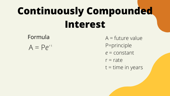 560×315 continuously compounding interest formula examples mathbootcamps from www.mathbootcamps.com
  295×237 complete table assuming continuously compounded interest initial from dejongbefornes.blogspot.com
  728×546 notes life compounding continuously from www.slideshare.net
 :max_bytes(150000):strip_icc()/ContinuousCompoundInterest4-e6827783080042dcac61083db9d7ae60.png) 6251×3959 continuous compound interest from www.investopedia.com
6251×3959 continuous compound interest from www.investopedia.com  728×546 calculate continuously compound interest from www.slideshare.net
  180×234 comparing investment options monthly compounded continuous from www.coursehero.com
  1024×768 chapter mathematics finance powerpoint from www.slideserve.com
  1280×720 continuously compounded interest youtube from www.youtube.com
  0 x 0 compounding interest continuously youtube from www.youtube.com
  1280×720 continuous compound interest youtube from www.youtube.com
  0 x 0 interest compounded continuously youtube from www.youtube.com
  1280×720 compound interest continuously youtube from www.youtube.com
